CarlAnomaly contains synchronized multi-modal autonomous-driving scenarios generated in CARLA, with train, normal test, and anomaly test splits.
| Split | Scenarios | Timesteps | Towns | Anomaly types |
|---|---|---|---|---|
| Train | 101 | 303,000 | 6 | 0 |
| Test normal | 107 | 32,100 | 6 | 0 |
| Test anomaly | 520 | 156,000 | 6 | 9 |
Sensor Setup
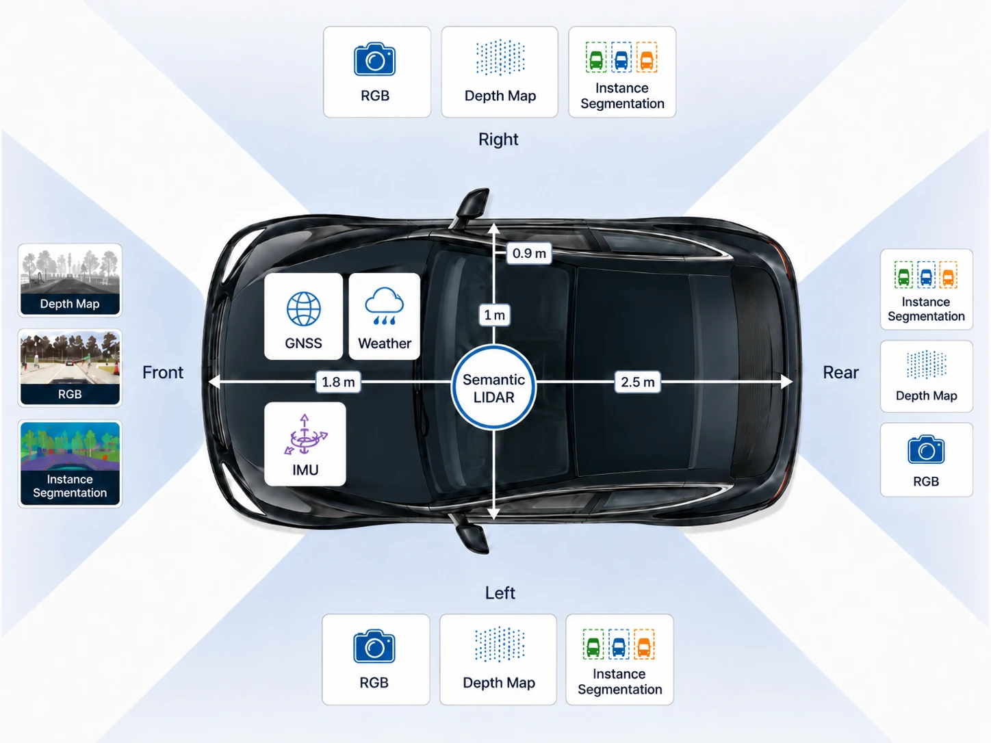
For data collection, we attached an array of sensors to the simulated vehicle.
On each of the 4 sides, front, left, right, rear, we attached virtual camera sensors that capture RGB-D data and instance segmentation masks.
Additionally, there is a LiDAR and a GNSS sensor at the center of the vehicle, as well as an IMU.
Furthermore, we capture the weather from the environment, as well as the control commands issued by
CARLA’s autopilot.
Anomaly Types
The test split contains nine anomaly types across four categories. Anomalies with a pixel mask can be evaluated at all four tiers (sample, sensor, timestep, scenario); those without a mask are only evaluated at the timestep and scenario levels.
| Category | Anomaly | Pixel Mask | Description |
|---|---|---|---|
| Unknown object | Turned-off traffic lights | ✓ | Traffic lights turn off, which never occurs in training scenarios. |
| Contextual | Debris spawn | ✓ | Known objects suddenly appear on the road in front of the ego vehicle. |
| Covariate / Temporal | Streetlight flickering | — | Streetlights flicker rapidly, altering night-time illumination. |
| Temporal | Vanish actor | — | A regularly driving vehicle disappears without physical cause. |
| Instant weather change | — | Weather conditions change abruptly within a few timesteps. | |
| Traffic light flickering | ✓ | Traffic lights alternate erratically between red and green. | |
| Traffic light yellow blinking | ✓ | Traffic lights continuously blink yellow, resembling a failure mode. | |
| Erratic driver | ✓ | A car abruptly steers without apparent reason. | |
| Running pedestrian | ✓ | A pedestrian moves at unusually high speed. |
Environmental Conditions
Scenarios span six CARLA towns (Town01–Town05, Town10HD) under diverse lighting and weather. Three base configurations cover clear, rainy, and foggy conditions; random interpolations between pairs produce a continuous range of atmospheric settings. Weather remains constant within each training scenario; abrupt weather transitions appear only in the test split as a dedicated temporal anomaly type.
Directory Structure
Scenarios are grouped by split and CARLA town (Town01–Town05, Town10HD). In the anomaly test split, scenarios are additionally grouped by anomaly type (e.g. change-weather, vanish-actor).
carlanomaly/
├── train/
│   ├── Town01/
│   │   ├── scenario-1/
│   │   └── ...
│   └── ...
└── test/
    ├── normal/
    │   ├── Town01/
    │   │   ├── scenario-1/
    │   │   └── ...
    │   └── ...
    └── anomaly/
        ├── Town01/
        │   ├── <anomaly-type>/
        │   │   ├── scenario-1/
        │   │   └── ...
        │   └── ...
        └── ...
Cameras
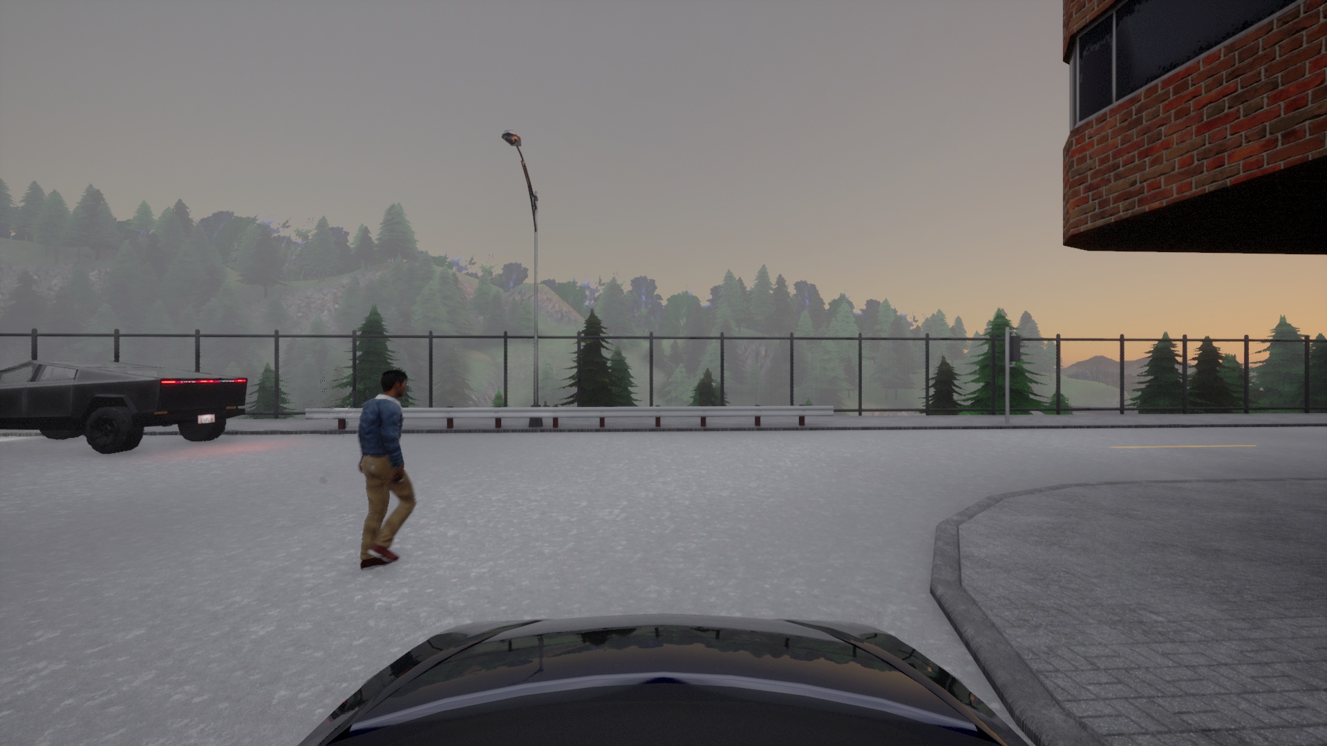
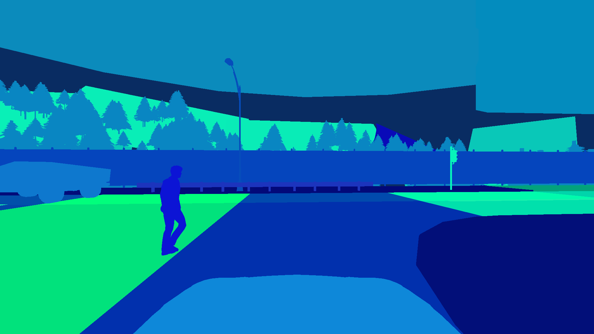
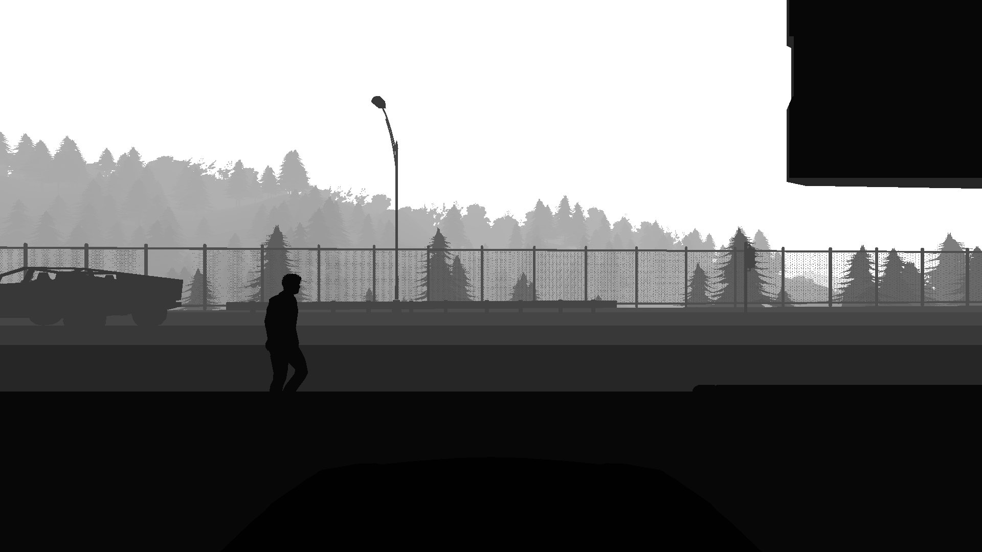
The dataset contains pixel- and instance wise segmentation masks for each object in the scene. Each object has a unique ID. Since these annotations were generated in a simulation, the annotations are perfect.
scenario/
├── rgb-front/
│   ├── 000000.jpg
│   └── ...
├── segmentation-front/
│   ├── 000000.png
│   └── ...
└── depth-front/
    ├── 000000.png
    └── ...
The instance segmentation masks can be loaded as follows:
img = Image.open("segmentation-front/000099.png")

# instance ids are encoded in the G and B channel
id_fields = np.array(img)[:,:,1:3]
instance_ids = np.zeros(shape=(id_fields.shape[0], id_fields.shape[1]), dtype=np.int32)
instance_ids += id_fields[:,:,0]
instance_ids += id_fields[:,:,1].astype(np.int32) << 8

# per-pixel classes are encoded in the R channel
segmentation_mask = np.array(img)[:,:,0]
Semantic LiDAR
Pixel-Annotated LiDAR point clouds for each timestep with realistic settings.
scenario/
└── pointclouds/
    ├── 000000.feather
    └── ...
These files can be loaded with pandas:
import pandas as pd
# Columns: x, y, z, angle, object_id, class_id
data = pd.read_feather("000000.feather")
KITTI Annotations
KITTI annotations contain 3D bounding boxes and connect them to the camera.
scenario/
└── kitti-front/
    ├── complete_data/
    │   ├── 000000_extended.json
    │   └── ...
    ├── label_2/
    │   ├── 000000.txt
    │   └── ...
    └── calib/
        ├── 000000.txt
        └── ...
Anomaly Annotations
In the CarlAnomaly dataset, anomaly detection can be done on several different levels.
Sample Level
For cameras the per-pixel anomaly labels are available in a separate directory. Labels are written in a 1-channel PNG where 0 means normal and everything else means anomaly.
scenario/
└── anomaly-front/
    ├── 000000.png
    ├── ...
For LiDAR the anomaly labels are similarly available in a separate directory:
scenario/
└── anomaly-lidar/
    ├── 000000.feather
    ├── ...
The .feather files are serialized dataframes with a column for the anomaly label.
Sensor Level
Sensor-level anomaly labels are given in a .feather file with an anomaly column.
scenario/
└── anomaly-front/
    ├── ...
    └── sensor.feather
└── anomaly-lidar/
    ├── ...
    └── sensor.feather
Timestep Level
A timestep is anomalous when any sensor reading at that point in time contains an anomaly. For convenience, these labels are also stored in feather format:
scenario/
└── anomaly-observation.feather
The columns are:
anomaly: True or Falsetick: Current timestep numberanomaly_obj_ids: List of objects ids for objects considered as anomaliesanomaly_class_ids: List of class ids for objects considered as anomaliesmeta: Metadata
Scenario Level
These labels are given by the directory.
Additional Data
The dataset additionally contains sensor readings for the following sensors in feather format:
- IMU: Measuring acceleration and orientation of the ego vehicle
- GNSS: Measuring position of the vehicle
- Weather: Exact weather conditions
- Actions: Actions executed by the auto-pilot (Note: these are the actions that are executed by CARLAs traffic manager after the last timestep)
- Collisions: List of collision events. There can be multiple collisions per timestep.
scenario/
├── gnss.feather
├── imu.feather
├── weather.feather
├── collisions.feather
└── actions.feather
You can simply load these as pandas dataframes.
Example: IMU
import pandas as pd
imu = pd.read_feather("imu.feather")
The per-timestep IMU readings look as follows: